Introduction to microbiomeutilities
Source:vignettes/microbiomeutilities.Rmd
microbiomeutilities.RmdNOTE While we continue to maintain this R package, the development has been discontinued as we have shifted to supporting methods development based on the new TreeSummarizedExperiment data container, which provides added capabilities for multi-omics data analysis. Check the miaverse project for details.
The microbiomeutilities R package is part of the microbiome-verse tools that
provides additional data handling and visualization support for the microbiome R/BioC
package
Philosophy: “Seemingly simple tasks for experienced R users can always be further simplified for novice users”
Install
install.packages("devtools")
devtools::install_github("microsud/microbiomeutilities")
Load libraries
Basics
Example data
Package data from Zackular et al., 2014: The Gut Microbiome Modulates Colon Tumorigenesis.
Import test data.
data("zackular2014")
ps0 <- zackular2014
ps0
#> phyloseq-class experiment-level object
#> otu_table()   OTU Table:         [ 2078 taxa and 88 samples ]
#> sample_data() Sample Data:       [ 88 samples by 7 sample variables ]
#> tax_table()   Taxonomy Table:    [ 2078 taxa by 7 taxonomic ranks ]
The print_ps from microbiomeutilities can
give additional information. See also
microbiome::summarize_phyloseq.
print_ps(ps0)
#> 01] ntaxa = 2078
#> 02] nsamples = 88
#> 03] nsamplesvariables = 7
#> 04] nranks = 7
#> 05] Min. number of reads = 15704
#> 06] Max. number of reads = 216888
#> 07] Total number of reads = 4594626
#> 08] Average number of reads = 52211.66
#> 09] Median number of reads = 49415.5
#> 10] Sparsity = 0.728426590252865
#> 11] Number of singletons = 0
#> 12] % of taxa that are singletons
#>   (i.e. exactly one read detected across all samples) = 0
Formatting the Phyloseq Object
Most commonly it is observed that the taxonomy file has classification until a given taxonomic level. We can change the names in both otu table and taxonomy table with the best taxonomic classification available. This can be useful if the analysis has to be done at OTU/ASVs level. Only ID are less useful.
Check the taxonomy in phyloseq object.
| Domain | Phylum | Class | Order | Family | Genus | Species | |
|---|---|---|---|---|---|---|---|
| d__denovo1773 | k__Bacteria | p__Bacteroidetes | c__Bacteroidia | o__Bacteroidales | f__Bacteroidaceae | g__Bacteroides | s__ |
| d__denovo1771 | k__Bacteria | p__Bacteroidetes | c__Bacteroidia | o__Bacteroidales | f__Bacteroidaceae | g__Bacteroides | s__ |
| d__denovo1776 | k__Bacteria | p__Firmicutes | c__Clostridia | o__Clostridiales | f__Ruminococcaceae | g__ | s__ |
| d__denovo1777 | k__Bacteria | p__Bacteroidetes | c__Bacteroidia | o__Bacteroidales | f__Bacteroidaceae | g__Bacteroides | s__ |
| d__denovo1775 | k__Bacteria | p__Firmicutes | c__Clostridia | o__Clostridiales | f__Lachnospiraceae | g__Blautia | s__ |
| d__denovo2639 | k__Bacteria | p__Bacteroidetes | c__Bacteroidia | o__Bacteroidales | f__Bacteroidaceae | g__Bacteroides | s__ |
Some have only g__ of s__ information.
data("zackular2014")
p0 <- zackular2014
# reduce size for example
ps0 <- core(p0, detection = 10, prevalence = 20 / 100)
# Add a prefix to taxa labels
ps0.f2 <- format_to_besthit(ps0, prefix = "MyBug-")

kable(head(tax_table(ps0.f2))[3:6])| Domain | Phylum | Class | Order | Family | Genus | Species | best_hit | |
|---|---|---|---|---|---|---|---|---|
| MyBug-d__denovo165:f__Ruminococcaceae | Bacteria | Firmicutes | Clostridia | Clostridiales | Ruminococcaceae | f__Ruminococcaceae | f__Ruminococcaceae | MyBug-d__denovo165:f__Ruminococcaceae |
| MyBug-d__denovo167:g__Coprococcus | Bacteria | Firmicutes | Clostridia | Clostridiales | Lachnospiraceae | Coprococcus | g__Coprococcus | MyBug-d__denovo167:g__Coprococcus |
| MyBug-d__denovo166:o__Clostridiales | Bacteria | Firmicutes | Clostridia | Clostridiales | o__Clostridiales | o__Clostridiales | o__Clostridiales | MyBug-d__denovo166:o__Clostridiales |
| MyBug-d__denovo161:g__Roseburia | Bacteria | Firmicutes | Clostridia | Clostridiales | Lachnospiraceae | Roseburia | g__Roseburia | MyBug-d__denovo161:g__Roseburia |
Now the available taxonomy is added.
As can be seen, the rownames have the OTUIDs and available taxonomic name(s).
Distribution of reads
Useful for QC purposes. Check for distribution of sequencing depth.
data("zackular2014")
p0 <- zackular2014
p <- plot_read_distribution(p0, groups = "DiseaseState",
                            plot.type = "density")
print(p + theme_biome_utils())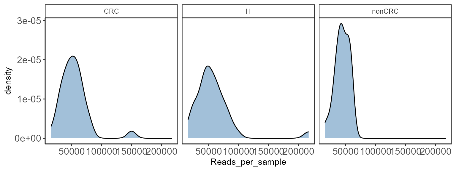
This is a diagnostic step. Key to check if there is variation between groups that will be compared for downstream analysis.
Convert phyloseq object to long data format
Useful if the user wants to plot specific features.
Converting to long data format opens several opportunities to work with
Tidyverse.
data("zackular2014")
p0 <- zackular2014
# reduce size for example
ps0 <- core(p0, detection = 10, prevalence = 20 / 100)

pseq_df <- phy_to_ldf(ps0, transform.counts = NULL)
#> An additonal column Sam_rep with sample names is created for reference purpose

kable(head(pseq_df))| OTUID | Domain | Phylum | Class | Order | Family | Genus | Species | Sam_rep | Abundance | investigation_type | project_name | DiseaseState | age | body_product | FOBT.result | material |
|---|---|---|---|---|---|---|---|---|---|---|---|---|---|---|---|---|
| d__denovo66 | k__Bacteria | p__Firmicutes | c__Clostridia | o__Clostridiales | f__Lachnospiraceae | g__Ruminococcus2 | s__ | Adenoma10-2757 | 27 | metagenomic | The Gut Microbiome Improves Predictive Models for Diagnosis of Colorectal Cancer | nonCRC | 37 | feces | negative | feces |
| d__denovo175 | k__Bacteria | p__Bacteroidetes | c__Bacteroidia | o__Bacteroidales | f__Rikenellaceae | g__Alistipes | s__ | Adenoma10-2757 | 0 | metagenomic | The Gut Microbiome Improves Predictive Models for Diagnosis of Colorectal Cancer | nonCRC | 37 | feces | negative | feces |
| d__denovo165 | k__Bacteria | p__Firmicutes | c__Clostridia | o__Clostridiales | f__Ruminococcaceae | g__ | s__ | Adenoma10-2757 | 49 | metagenomic | The Gut Microbiome Improves Predictive Models for Diagnosis of Colorectal Cancer | nonCRC | 37 | feces | negative | feces |
| d__denovo167 | k__Bacteria | p__Firmicutes | c__Clostridia | o__Clostridiales | f__Lachnospiraceae | g__Coprococcus | s__ | Adenoma10-2757 | 155 | metagenomic | The Gut Microbiome Improves Predictive Models for Diagnosis of Colorectal Cancer | nonCRC | 37 | feces | negative | feces |
| d__denovo166 | k__Bacteria | p__Firmicutes | c__Clostridia | o__Clostridiales | f__ | g__ | s__ | Adenoma10-2757 | 0 | metagenomic | The Gut Microbiome Improves Predictive Models for Diagnosis of Colorectal Cancer | nonCRC | 37 | feces | negative | feces |
| d__denovo161 | k__Bacteria | p__Firmicutes | c__Clostridia | o__Clostridiales | f__Lachnospiraceae | g__Roseburia | s__ | Adenoma10-2757 | 11 | metagenomic | The Gut Microbiome Improves Predictive Models for Diagnosis of Colorectal Cancer | nonCRC | 37 | feces | negative | feces |
Taxa overview
One of the first questions arise regarding which taxa are present , how they are distributed in the data. This can be done with following functionality.
Check distribution
A quick check to see how different taxa are distributed in your data.
library(microbiomeutilities)
library(RColorBrewer)
library(patchwork)
library(ggpubr)
data("zackular2014")
pseq <- zackular2014

# check healthy
health_ps <- subset_samples(pseq, DiseaseState=="H")
p_hc <- taxa_distribution(health_ps) +
  theme_biome_utils() +
  labs(title = "Healthy")

# check CRC
crc_ps <- subset_samples(pseq, DiseaseState=="CRC")
p_crc <- taxa_distribution(crc_ps) +
  theme_biome_utils() +
  labs(title = "CRC")

# harnessing the power of patchwork
p_hc / p_crc + plot_layout(guides = "collect") +
  plot_annotation(tag_levels = "A")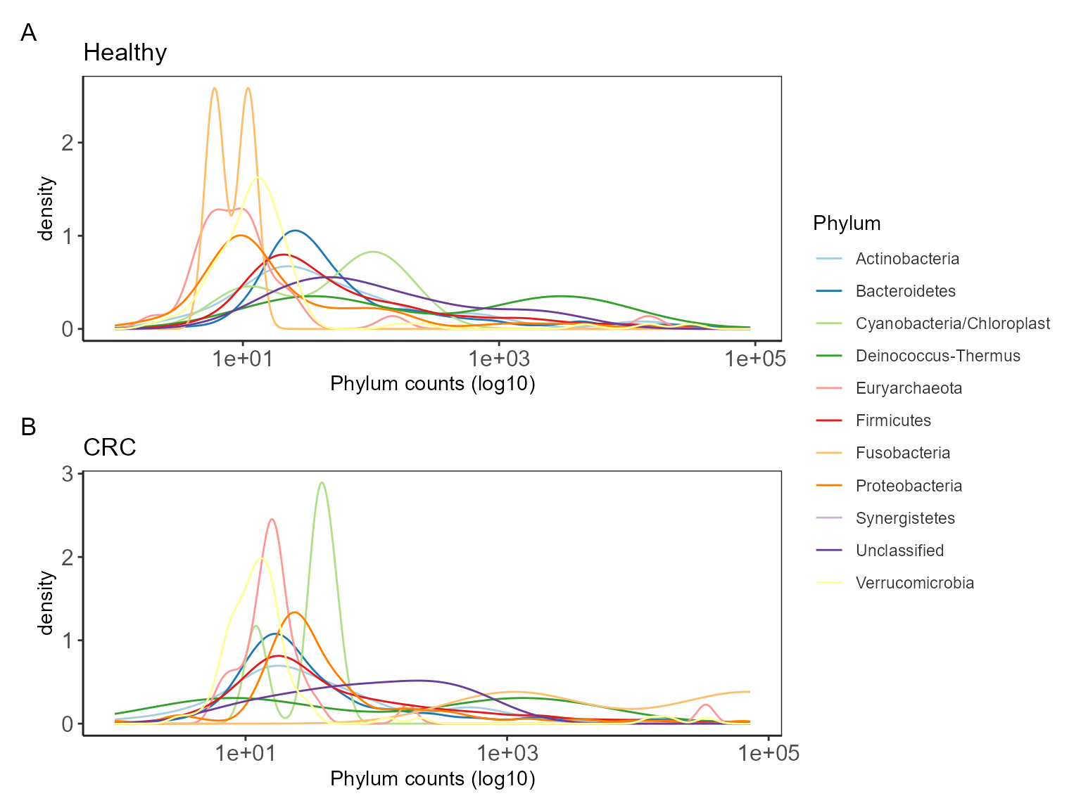
There are Cyanobacteria/Chloroplast related sequences which can be removed if not expected in the samples.
Dominant taxa
Sometimes, we are interested in identifying the most dominant taxa in each sample. We may also wish to check what percent of samples within a given group are these taxa dominating.
library(microbiomeutilities)
library(dplyr)
data("zackular2014")
p0 <- zackular2014
p0.gen <- aggregate_taxa(p0,"Genus")
x.d <- dominant_taxa(p0,level = "Genus", group="DiseaseState")
head(x.d$dominant_overview)
#> # A tibble: 6 × 5
#> # Groups:   DiseaseState [3]
#>   DiseaseState dominant_taxa      n rel.freq rel.freq.pct
#>   <fct>        <chr>          <int>    <dbl> <chr>
#> 1 H            g__Bacteroides    15     50   50%
#> 2 nonCRC       g__Blautia        13     46.4 46%
#> 3 CRC          g__Bacteroides     9     30   30%
#> 4 CRC          g__Blautia         9     30   30%
#> 5 H            g__Blautia         7     23.3 23%
#> 6 nonCRC       g__Bacteroides     6     21.4 21%
As seen in the table above, 50% of the samples in H
group are dominated by *g__Bacteroides* and so on…
Get taxa summary
This can be used for entire dataset.
library(microbiomeutilities)
data("zackular2014")
p0 <- zackular2014
tx.sum1 <- taxa_summary(p0, "Phylum")
#> Data provided is not compositional
#>  will first transform
tx.sum1
#>                            Taxa          Max.Rel.Ab          Mean.Rel.Ab
#> 1              p__Euryarchaeota   0.218508035656191   0.0200267274400673
#> 2                           p__  0.0359956743395643  0.00213630393381328
#> 3             p__Actinobacteria   0.189937172231165   0.0294096453288836
#> 4              p__Bacteroidetes   0.703769740193581    0.244709411770076
#> 5  p__Cyanobacteria/Chloroplast 0.00391786546652736 0.000248991452140149
#> 6        p__Deinococcus-Thermus  0.0306807689079157  0.00136619388828292
#> 7                 p__Firmicutes   0.935779308307329    0.609116019352896
#> 8               p__Fusobacteria   0.390135934239562   0.0079458294240542
#> 9             p__Proteobacteria   0.403932082216265     0.04116346455827
#> 10             p__Synergistetes  0.0106576610162058 0.000207008030950549
#> 11           p__Verrucomicrobia   0.320077232101149   0.0436704048205656
#>           Median.Rel.Ab             Std.dev
#> 1  4.08341966447163e-05  0.0445500008069431
#> 2  0.000335981950200747 0.00577447214134393
#> 3    0.0152970058974793  0.0361457627428506
#> 4     0.193736718210234   0.183986562646175
#> 5  2.58996131628288e-05 0.00070384339925814
#> 6                     0 0.00449398785197828
#> 7     0.598709982286244   0.182320763133074
#> 8                     0  0.0514603201611758
#> 9    0.0130121759294526  0.0774502267516943
#> 10                    0 0.00119199461324549
#> 11  0.00665688163392832  0.0679829229763011
Get taxa summary by group(s)
For group specific abundances of taxa
get_group_abundances.
library(microbiomeutilities)
data("zackular2014")
p0 <- zackular2014
grp_abund <- get_group_abundances(p0,
                                  level = "Phylum",
                                  group="DiseaseState",
                                  transform = "compositional")
How to visualize these data?
mycols <- c("brown3", "steelblue","grey50")

# clean names
grp_abund$OTUID <- gsub("p__", "",grp_abund$OTUID)
grp_abund$OTUID <- ifelse(grp_abund$OTUID == "",
                          "Unclassified", grp_abund$OTUID)


mean.plot <- grp_abund %>% # input data
  ggplot(aes(x= reorder(OTUID, mean_abundance), # reroder based on mean abundance
             y= mean_abundance,
             fill=DiseaseState)) + # x and y axis
  geom_bar(     stat = "identity",
                position=position_dodge()) +
  scale_fill_manual("DiseaseState", values=mycols) + # manually specify colors
  theme_bw() + # add a widely used ggplot2 theme
  ylab("Mean Relative Abundance") + # label y axis
  xlab("Phylum") + # label x axis
  coord_flip() # rotate plot

mean.plot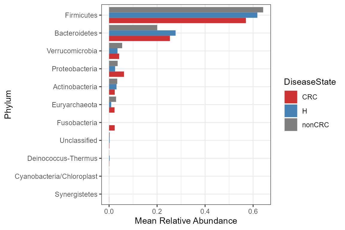
This plot is diagnostic to have an idea about the taxonomy in each group. Statements based on comparisons between groups may not make sense here because only mean abundance values are plotted, and not standard deviation within groups. For visualizing error bars and more check Statistical tools for high-throughput data analysis.
Find samples dominated by specific taxa
Finding samples dominated by user provided taxa in a phyloseq object. This is useful especially if user suspects a taxa to be contaminant and wishes to identify which samples are dominated by the contaminant taxa.
library(microbiomeutilities)
data("zackular2014")
p0 <- zackular2014
p0.f <- aggregate_taxa(p0, "Genus")
bac_dom <- find_samples_taxa(p0.f, taxa = "g__Bacteroides")
bac_dom
#>  [1] "Adenoma14-2817"    "Adenoma20-2995"    "Adenoma21-3129"
#>  [4] "Adenoma22-3133"    "Adenoma24-3217"    "Adenoma9-2717"
#>  [7] "Cancer10-2567"     "Cancer11-2573"     "Cancer1-2355"
#> [10] "Cancer17-2625"     "Cancer20-2667"     "Cancer22-2703"
#> [13] "Cancer30-2863"     "Cancer5-2523"      "Cancer9-2547"
#> [16] "Healthy10-3087"    "Healthy11-3123"    "Healthy1-2027"
#> [19] "Healthy13-3241"    "Healthy14-3245"    "Healthy16-3251"
#> [22] "Healthy17-3257"    "Healthy18-3293"    "Healthy19-3339"
#> [25] "Healthy20-3341"    "Healthy26-3407"    "Healthy30-3291-66"
#> [28] "Healthy6-3061"     "Healthy8-3073"     "Healthy9-3075"

#get samples dominated by g__Bacteroides
ps.sub <- prune_samples(sample_names(p0.f) %in% bac_dom, p0.f)
Alpha diversity
Rarefaction curves for alpha diversity indices
A common approach to check for sequencing depth and diversity
measures.
Here, we can access the numerous alpha diversity measures supported by
microbiome
R package.
NOTE: This can take sometime to complete.
library(microbiomeutilities)
data("zackular2014")
p0 <- zackular2014
# set seed
set.seed(1)
subsamples <- seq(0, 5000, by=100)[-1]
#subsamples = c(10, 5000, 10000, 20000, 30000)

p <- plot_alpha_rcurve(p0, index="observed",
                       subsamples = subsamples,
                       lower.conf = 0.025,
                       upper.conf = 0.975,
                       group="DiseaseState",
                       label.color = "brown3",
                       label.size = 3,
                       label.min = TRUE)
# change color of line
mycols <- c("brown3", "steelblue","grey50")

p <- p + scale_color_manual(values = mycols) +
  scale_fill_manual(values = mycols)
print(p)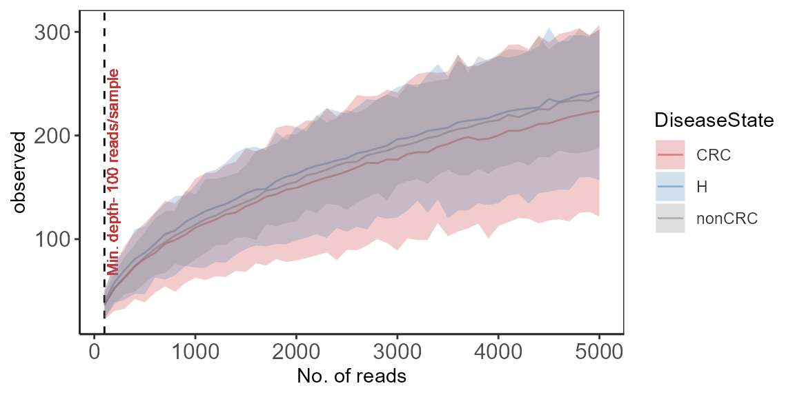
Plot alpha diversities
Utility plot function for diversity measures calculated by
microbiome package.
library(microbiome)
data("zackular2014")
ps0 <- zackular2014
mycols <- c("brown3", "steelblue","grey50")
p <- plot_alpha_diversities(ps0,
                            type = "dominance",
                            index.val = "all",
                            plot.type = "stripchart",
                            variableA = "DiseaseState",
                            palette = mycols)

p <- p + theme_biome_utils() +
  ggplot2::theme(legend.position = "top",
                 text = element_text(size=14))
print(p)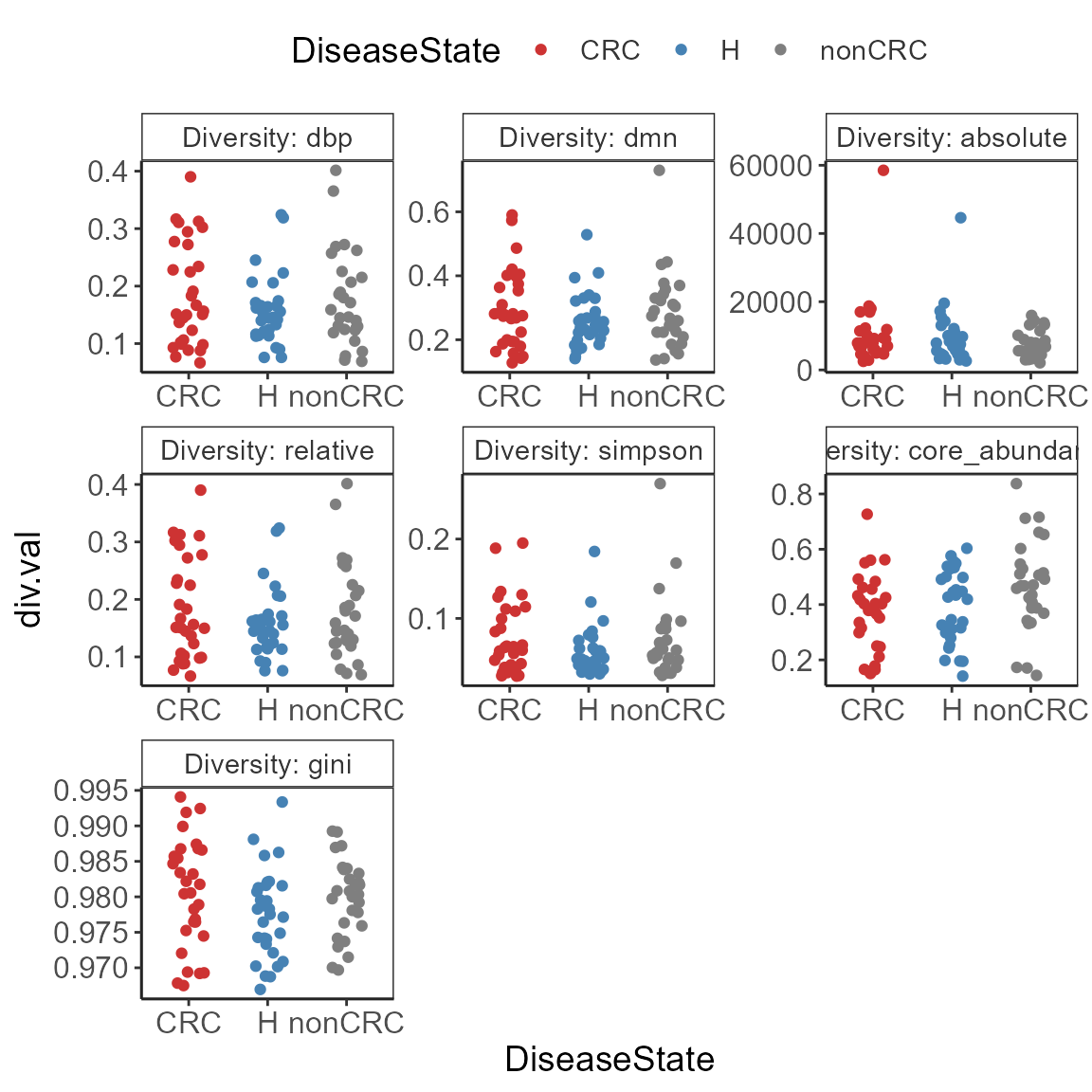
comps <- make_pairs(sample_data(ps0)$DiseaseState)

p <- p + stat_compare_means(
      comparisons = comps,
      label = "p.format",
      tip.length = 0.05,
      method = "wilcox.test")
p
#> Warning in wilcox.test.default(c(7855, 4967, 16964, 6997, 11425, 17013, : cannot
#> compute exact p-value with ties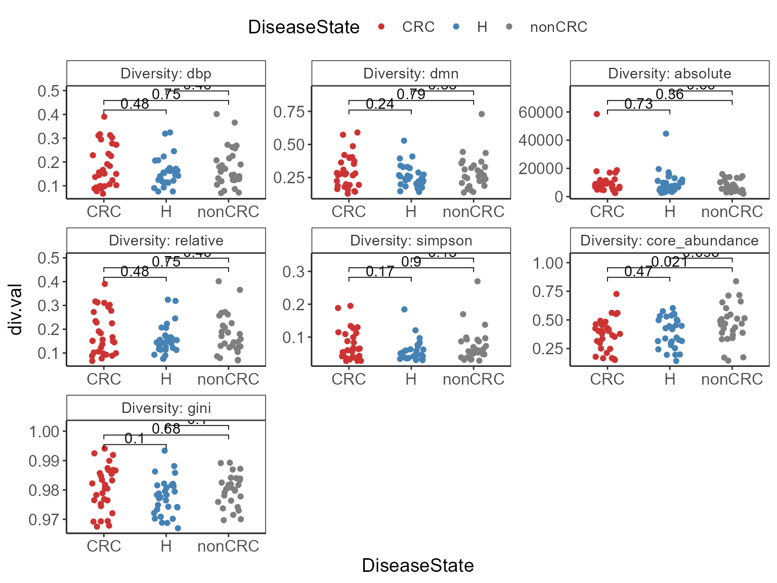
Alternatively, one can plot one index at a time with pair-wise stats.
library(gghalves)
library(microbiomeutilities)
data("zackular2014")
p0 <- zackular2014
mycols <- c("brown3", "steelblue","grey50")

p.m <- plot_diversity_stats(p0, group = "DiseaseState",
                            index = "diversity_shannon",
                            group.order = c("H", "CRC", "nonCRC"),
                            group.colors = mycols,
                            label.format="p.format",
                            stats = TRUE)
#> Warning: `guides(<scale> = FALSE)` is deprecated. Please use `guides(<scale> =
#> "none")` instead.
p.m + ylab("Shannon Diversity") + xlab("")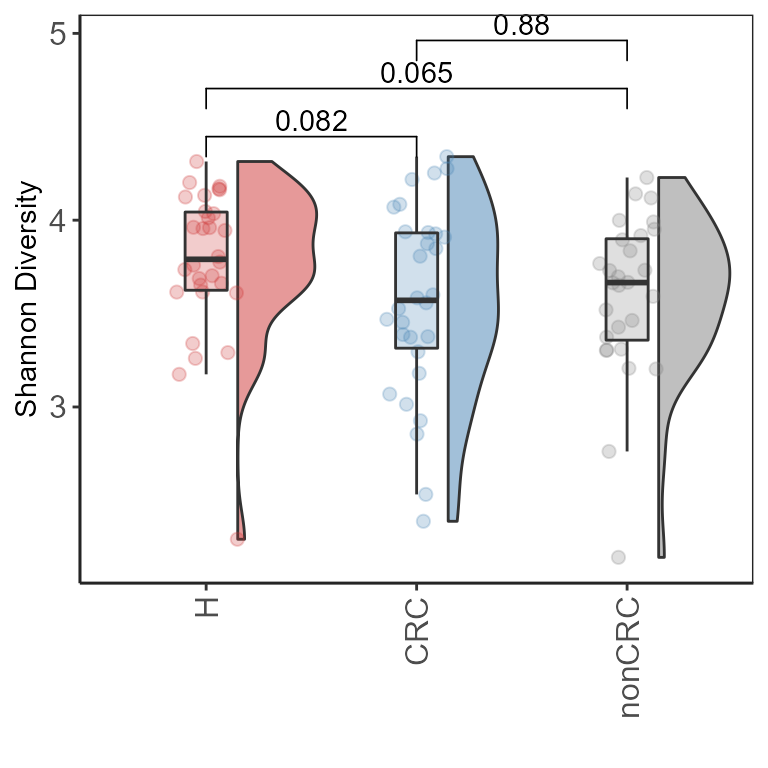
Composition plots
Ternary plot
library(microbiome)
library(microbiomeutilities)
library(dplyr)
data("zackular2014")
p0 <- zackular2014
tern_df <- prep_ternary(p0, group="DiseaseState",
               abund.thres=0.000001, level= "Genus", prev.thres=0.01)
head(tern_df)
#> # A tibble: 6 × 11
#> # Groups:   unique [6]
#>   unique         CRC      H  nonCRC Domain Phylum Class Order Family Genus OTUID
#>   <chr>        <dbl>  <dbl>   <dbl> <chr>  <chr>  <chr> <chr> <chr>  <chr> <chr>
#> 1 Acetanaer… 0.00995 0.0135 0.00858 Bacte… Firmi… Clos… Clos… Rumin… Acet… Acet…
#> 2 Acidamino… 0.115   0.164  0.0846  Bacte… Firmi… Nega… Sele… Acida… Acid… Acid…
#> 3 Acinetoba… 0.0108  0.0312 0.00762 Bacte… Prote… Gamm… Pseu… Morax… Acin… Acin…
#> 4 Actinomyc… 0.0169  0.0338 0.0218  Bacte… Actin… Acti… Acti… Actin… Acti… Acti…
#> 5 Akkermans… 1.26    1.05   1.53    Bacte… Verru… Verr… Verr… Verru… Akke… Akke…
#> 6 Alistipes  0.929   0.894  0.654   Bacte… Bacte… Bact… Bact… Riken… Alis… Alis…
# install.packages("ggtern")
require(ggtern)

# Replace empty with Other
tern_df$Phylum[tern_df$Phylum==""] <- "Other"

ggtern(data=tern_df, aes(x=CRC, y=H, z=nonCRC)) +
  geom_point(aes(color= Phylum),
             alpha=0.25,
             show.legend=T,
             size=3) +
  #scale_size(range=c(0, 6)) +
  geom_mask() +
  scale_colour_brewer(palette = "Paired") +
  theme_biome_utils()

detach("package:ggtern", unload=TRUE)
Plot taxa boxplot
Plot relative abundance of top taxa specified by user.
library(microbiomeutilities)
library(RColorBrewer)
data("zackular2014")
ps0 <- zackular2014
mycols <- c("brown3", "steelblue", "grey50")
pn <- plot_taxa_boxplot(ps0,
                        taxonomic.level = "Family",
                        top.otu = 3,
                        group = "DiseaseState",
                        add.violin= FALSE,
                        title = "Top three family",
                        keep.other = FALSE,
                        group.order = c("H","CRC","nonCRC"),
                        group.colors = mycols,
                        dot.size = 1)

print(pn + theme_biome_utils())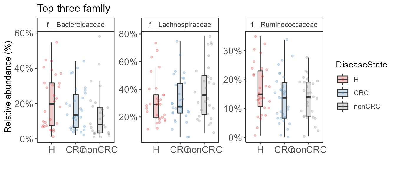
Plotting selected taxa
Using a list of taxa specified by the user for comparisons.
library(microbiome)
library(microbiomeutilities)
library(ggpubr)
data("zackular2014")
p0 <- zackular2014
p0.f <- format_to_besthit(p0)
#top_taxa(p0.f, 5)
select.taxa <- c("d__denovo1:g__Blautia", "d__denovo3:g__Bacteroides")

mycols <- c("brown3", "steelblue", "grey50")

p <- plot_listed_taxa(p0.f, select.taxa,
                      group= "DiseaseState",
                      group.order = c("H","CRC","nonCRC"),
                      group.colors = mycols,
                      add.violin = TRUE,
                      violin.opacity = 0.3,
                      dot.opacity = 0.25,
                      box.opacity = 0.25,
                      panel.arrange= "grid")
#> An additonal column Sam_rep with sample names is created for reference purpose
#> Warning: `guides(<scale> = FALSE)` is deprecated. Please use `guides(<scale> =
#> "none")` instead.
print(p + ylab("Relative abundance") + scale_y_continuous(labels = scales::percent))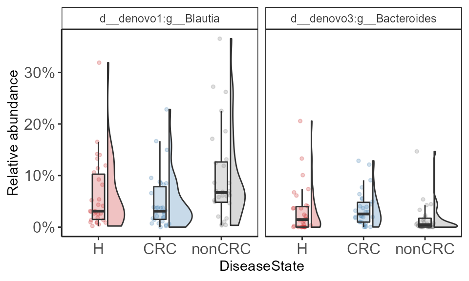
Adding statistical test with
ggpubr::stat_compare_means()
# If more than two variables
comps <- make_pairs(sample_data(p0.f)$DiseaseState)
print(comps)
#> [[1]]
#> [1] "CRC" "H"
#>
#> [[2]]
#> [1] "CRC"    "nonCRC"
#>
#> [[3]]
#> [1] "H"      "nonCRC"
p <- p + stat_compare_means(
      comparisons = comps,
      label = "p.format",
      tip.length = 0.05,
      method = "wilcox.test")
p + scale_y_continuous(labels = scales::percent)
#> Warning in wilcox.test.default(c(0.0737753988097334, 0.0369437665507036, :
#> cannot compute exact p-value with ties
#> Warning in wilcox.test.default(c(0.0218880793675399, 0.000317486610347303, :
#> cannot compute exact p-value with ties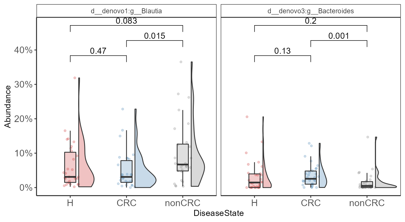
Plot top four Genera
library(microbiome)
library(microbiomeutilities)
data("zackular2014")
p0 <- zackular2014
p0.f <- aggregate_taxa(p0, "Genus")
top_four <- top_taxa(p0.f, 4)
top_four
#> [1] "g__Bacteroides"      "g__Blautia"          "g__Faecalibacterium"
#> [4] "g__Akkermansia"

mycols <- c("brown3", "steelblue", "grey50")

p <- plot_listed_taxa(p0.f, top_four,
                      group= "DiseaseState",
                      group.order = c("H","CRC","nonCRC"),
                      group.colors = mycols,
                      add.violin = TRUE,
                      violin.opacity = 0.3,
                      dot.opacity = 0.25,
                      box.opacity = 0.25,
                      panel.arrange= "wrap")
#> Warning: `guides(<scale> = FALSE)` is deprecated. Please use `guides(<scale> =
#> "none")` instead.

comps <- make_pairs(sample_data(p0.f)$DiseaseState)
p <- p + stat_compare_means(
      comparisons = comps,
      label = "p.format",
      tip.length = 0.05,
      method = "wilcox.test")

print(p + ylab("Relative abundance") + scale_y_continuous(labels = scales::percent))
#> Warning in wilcox.test.default(c(0.0242631263865901, 5.19237758969832e-05, :
#> cannot compute exact p-value with ties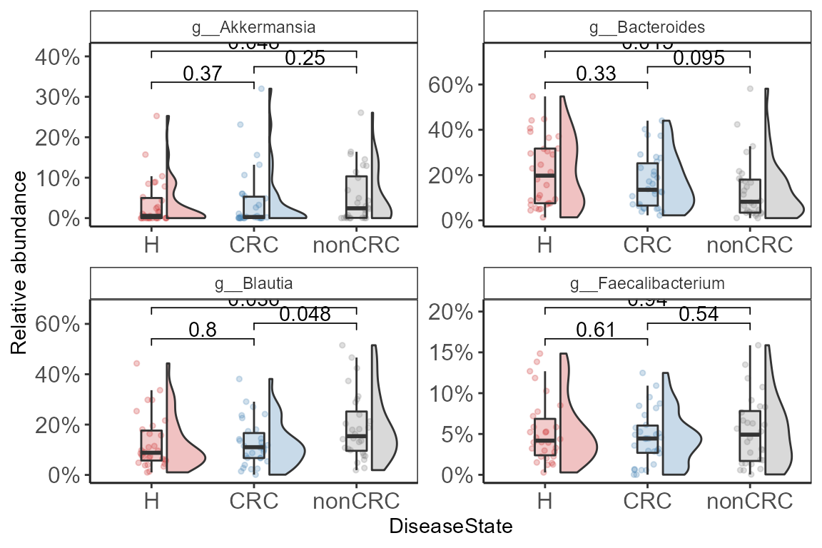
Abundance-Prevalence relationship
Plots mean Abundance-Prevalence for taxa. Mean abundance, mean
prevalence, and upper and lower confidence interval for each taxa is
calculated by random sub-sampling.
This can be useful in identifying highly prevalent taxa and their mean
relative abundance in a group of samples. Taxa that are highly prevalent
with low variation in lower and upper CI can be identified at varying
values of mean relative abundance. These are likely core taxa in the
groups of samples.
See core microbiota analysis in microbiome R package
library(microbiomeutilities)
library(dplyr)
library(ggrepel)
asv_ps <- zackular2014
asv_ps <- microbiome::transform(asv_ps, "compositional")
# Select healthy samples
asv_ps <- subset_samples(asv_ps, DiseaseState=="H")
asv_ps <- core(asv_ps,detection = 0.0001, prevalence = 0.50) # reduce size for example
asv_ps <- format_to_besthit(asv_ps)

set.seed(14285)
p_v <- plot_abund_prev(asv_ps,
                       label.core = TRUE,
                       color = "Phylum", # NA or "blue"
                       mean.abund.thres = 0.01,
                       mean.prev.thres = 0.99,
                       dot.opacity = 0.7,
                       label.size = 3,
                       label.opacity = 1.0,
                       nudge.label=-0.15,
                       bs.iter=9, # increase for actual analysis e.g. 999
                       size = 20, # increase to match your nsamples(asv_ps)
                       replace = TRUE,
                       label.color="#5f0f40")
p_v <- p_v +
  geom_vline(xintercept = 0.95, lty="dashed", alpha=0.7) +
  geom_hline(yintercept = 0.01,lty="dashed", alpha=0.7) +
  scale_color_brewer(palette = "Dark2")
p_v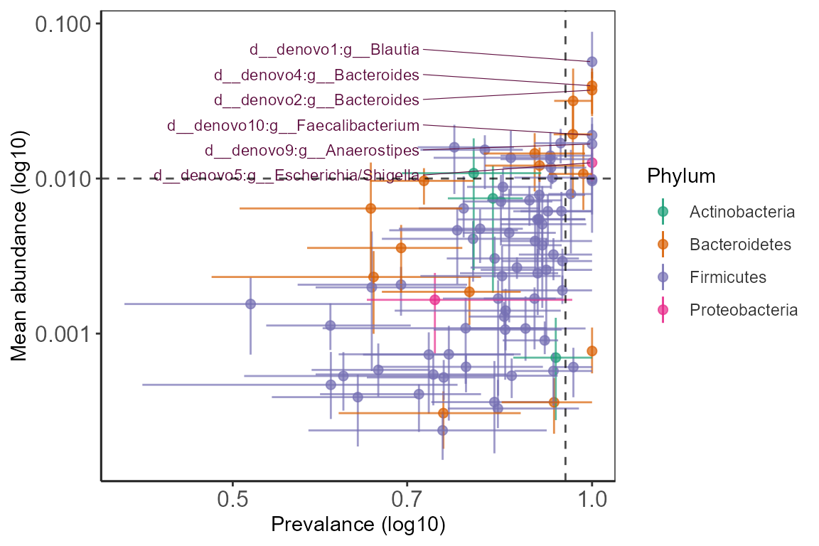
Heatmaps
Heatmap using phyloseq and pheatmap
Useful for visualizing differences in top OTUs between sample groups.
library(microbiomeutilities)
library(pheatmap)
library(RColorBrewer)
data("zackular2014")
ps0 <- zackular2014

#optional step if required to rename taxa_names
taxa_names(ps0) <- gsub("d__denovo", "OTU:", taxa_names(ps0))

# create a gradient color palette for abundance
grad_ab <- colorRampPalette(c("#faf3dd","#f7d486" ,"#5e6472"))
grad_ab_pal <- grad_ab(10)

# create a color palette for varaibles of interest
meta_colors <- list(c("positive" = "#FFC857",
                      "negative" = "#05B083"),
                    c("CRC" = "steelblue",
                      "nonCRC" = "grey50",
                      "H"="brown3"))
# add labels for pheatmap to detect
names(meta_colors) <- c("FOBT.result", "DiseaseState")

p <- plot_taxa_heatmap(ps0,
                       subset.top = 25,
                       VariableA = c("DiseaseState","FOBT.result"),
                       heatcolors = grad_ab_pal, #rev(brewer.pal(6, "RdPu")),
                       transformation = "log10",
                       cluster_rows = T,
                       cluster_cols = F,
                       show_colnames = F,
                       annotation_colors=meta_colors)
#> Top 25 OTUs selected
#> log10, if zeros in data then log10(1+x) will be used
#> First top taxa were selected and
#> then abundances tranformed to log10(1+X)
#> Warning in transform(phyobj1, "log10"): OTU table contains zeroes. Using log10(1
#> + x) transform.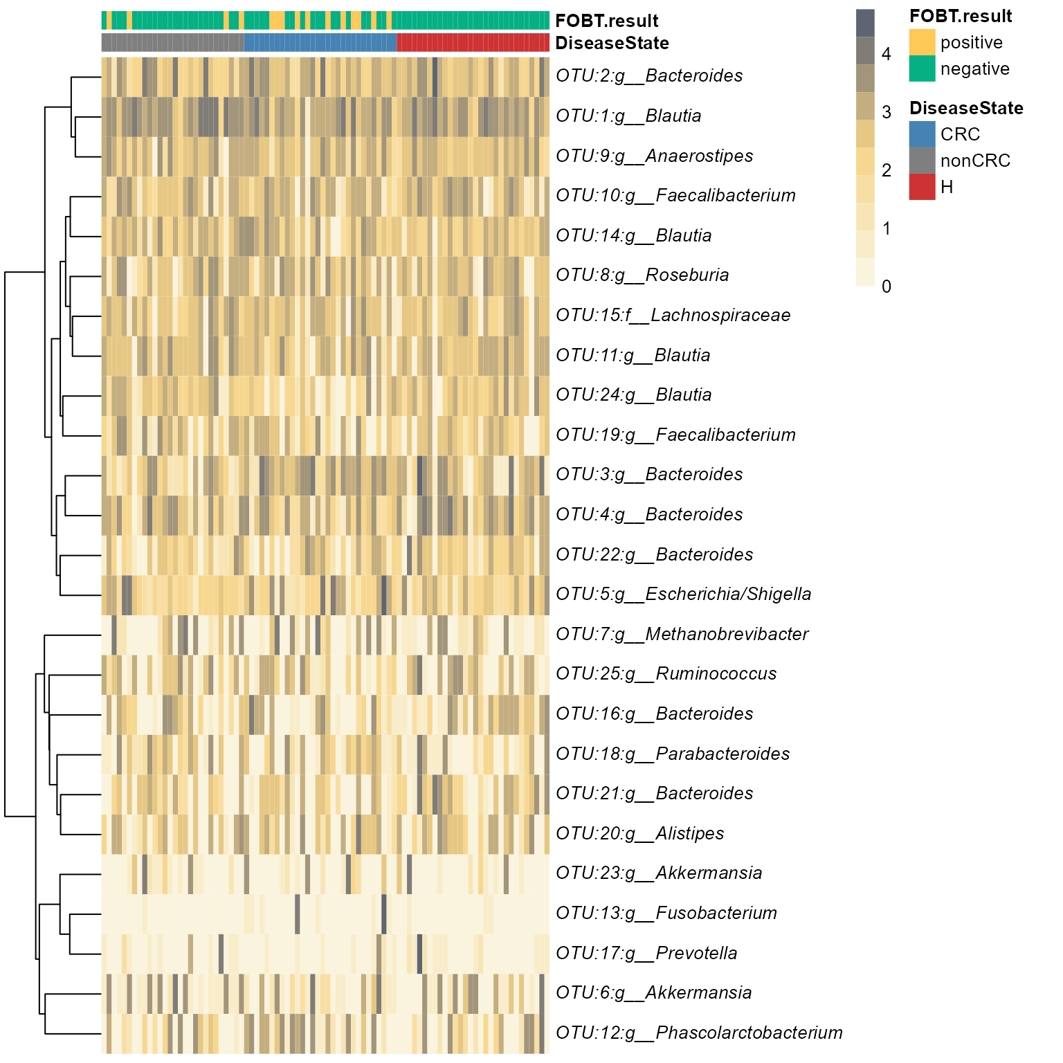
#the plot is stored here
p$plot

# table used for plot is here
p$tax_tab[1:3,1:3]
Elegant option with ggplot2
library(microbiomeutilities)
data("zackular2014")
p0 <- zackular2014
p0.rel <- transform(p0, "compositional")
#heat.cols <- c("#a8dadc","#457b9d", "#1d3557")
# create a gradient color palette for abundance
grad_ab <- colorRampPalette(c("#96d4ca","#d3f3f1", "#7c65a9"))
heat.cols <- grad_ab(10)
simple_heatmap(p0.rel,
               group.facet = "DiseaseState",
               group.order = NULL,
               abund.thres = 0.01,
               prev.thres = 0.1,
               level = "Genus",
               scale.color = "log10",
               na.fill = "white",
               color.fill = heat.cols,
               taxa.arrange=TRUE,
               remove.other=TRUE,
               panel.arrange="grid",
               ncol=NULL,
               nrow=NULL)
#> Warning: Transformation introduced infinite values in discrete y-axis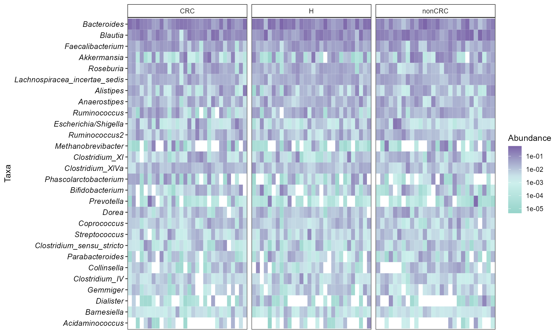
For heatmap options see microbiome::heat() and ampvis2
For other longitudinal related functionality check the [Longitudinal data analysis and visualization] section in the Articles section.
MicrobiomeHD datasets as phyloseq objects
We provide access to a subset of studies included in the
MicrobiomeHD database from Duvallet et al 2017: Meta-analysis
of gut microbiome studies identifies disease-specific and shared
responses. Nature communications.
The phyloseq objects are stored and accessed from microbiomedatarepo.
study <- list_microbiome_data(printtab = FALSE)

knitr::kable(study)
Below is the per study reference.
NOTE: When using these studies, please cite Duvallet et al. 2017 and the respective studies.
file <- system.file("extdata", "microbiomeHD_ref.txt", package = "microbiomeutilities")
reference <- read.table(file, header = T, sep = "\t")

knitr::kable(reference)
Experimental
Plot ordination and core
library(microbiomeutilities)
library(RColorBrewer)
data("zackular2014")
p0 <- zackular2014

ps1 <- format_to_besthit(p0)

#ps1 <- subset_samples(ps1, DiseaseState == "H")
ps1 <- prune_taxa(taxa_sums(ps1) > 0, ps1)
prev.thres <- seq(.05, 1, .05)
det.thres <- 10^seq(log10(1e-4), log10(.2), length = 10)
pseq.rel <- microbiome::transform(ps1, "compositional")
# reduce size for example
pseq.rel <- core(pseq.rel, detection = 0.001, prevalence = 20 / 100)

ord.bray <- ordinate(pseq.rel, "NMDS", "bray")

p <- plot_ordiplot_core(pseq.rel, ord.bray,
                        prev.thres, det.thres,
                        min.prevalence = 0.9,
                        color.opt = "DiseaseState",
                        shape = NULL, Sample = TRUE)

print(p)
Useful resources:
The microbiomeutilties depends on the phyloseq data
structure and core Phyloseq functions.
Tools for microbiome analysis in R. Microbiome package URL: microbiome package.
For more tutorials and examples of data analysis in R please check:
Contributions are welcome:
Issue
Tracker
Pull
requests
Star us on the
Github page
sessionInfo()
#> R version 4.2.1 (2022-06-23 ucrt)
#> Platform: x86_64-w64-mingw32/x64 (64-bit)
#> Running under: Windows 10 x64 (build 19044)
#>
#> Matrix products: default
#>
#> locale:
#> [1] LC_COLLATE=English_United States.utf8
#> [2] LC_CTYPE=English_United States.utf8
#> [3] LC_MONETARY=English_United States.utf8
#> [4] LC_NUMERIC=C
#> [5] LC_TIME=English_United States.utf8
#>
#> attached base packages:
#> [1] stats     graphics  grDevices utils     datasets  methods   base
#>
#> other attached packages:
#>  [1] pheatmap_1.0.12             ggrepel_0.9.1
#>  [3] gghalves_0.1.3              ggpubr_0.4.0
#>  [5] patchwork_1.1.2             RColorBrewer_1.1-3
#>  [7] tibble_3.1.7                knitr_1.40
#>  [9] microbiomeutilities_1.00.16 dplyr_1.0.9
#> [11] microbiome_1.18.0           ggplot2_3.3.6
#> [13] phyloseq_1.40.0
#>
#> loaded via a namespace (and not attached):
#>  [1] nlme_3.1-157           bitops_1.0-7           fs_1.5.2
#>  [4] rprojroot_2.0.3        GenomeInfoDb_1.32.2    backports_1.4.1
#>  [7] tools_4.2.1            bslib_0.4.0            utf8_1.2.2
#> [10] R6_2.5.1               vegan_2.6-2            DBI_1.1.3
#> [13] BiocGenerics_0.42.0    mgcv_1.8-40            colorspace_2.0-3
#> [16] permute_0.9-7          rhdf5filters_1.8.0     ade4_1.7-19
#> [19] withr_2.5.0            tidyselect_1.1.2       compiler_4.2.1
#> [22] textshaping_0.3.6      cli_3.3.0              Biobase_2.56.0
#> [25] desc_1.4.2             labeling_0.4.2         sass_0.4.2
#> [28] scales_1.2.1           pkgdown_2.0.6          systemfonts_1.0.4
#> [31] stringr_1.4.1          digest_0.6.29          rmarkdown_2.16
#> [34] XVector_0.36.0         pkgconfig_2.0.3        htmltools_0.5.3
#> [37] highr_0.9              fastmap_1.1.0          rlang_1.0.5
#> [40] rstudioapi_0.14        farver_2.1.1           jquerylib_0.1.4
#> [43] generics_0.1.3         jsonlite_1.8.0         car_3.1-0
#> [46] RCurl_1.98-1.6         magrittr_2.0.3         GenomeInfoDbData_1.2.8
#> [49] biomformat_1.24.0      Matrix_1.5-1           Rcpp_1.0.8.3
#> [52] munsell_0.5.0          S4Vectors_0.34.0       Rhdf5lib_1.18.2
#> [55] fansi_1.0.3            abind_1.4-5            ape_5.6-2
#> [58] lifecycle_1.0.2        stringi_1.7.6          yaml_2.3.5
#> [61] carData_3.0-5          MASS_7.3-57            zlibbioc_1.42.0
#> [64] rhdf5_2.40.0           Rtsne_0.16             plyr_1.8.7
#> [67] grid_4.2.1             parallel_4.2.1         crayon_1.5.1
#> [70] lattice_0.20-45        Biostrings_2.64.0      splines_4.2.1
#> [73] multtest_2.52.0        pillar_1.8.1           igraph_1.3.1
#> [76] ggsignif_0.6.3         reshape2_1.4.4         codetools_0.2-18
#> [79] stats4_4.2.1           glue_1.6.2             evaluate_0.16
#> [82] data.table_1.14.2      vctrs_0.4.1            foreach_1.5.2
#> [85] gtable_0.3.1           purrr_0.3.4            tidyr_1.2.0
#> [88] assertthat_0.2.1       cachem_1.0.6           xfun_0.31
#> [91] broom_1.0.1            rstatix_0.7.0          ragg_1.2.2
#> [94] survival_3.3-1         iterators_1.0.14       memoise_2.0.1
#> [97] IRanges_2.30.0         cluster_2.1.3          ellipsis_0.3.2