Longitudinal data analysis and visualization
Source:vignettes/microbiomeutilities_ts.Rmd
microbiomeutilities_ts.RmdLongitudinal data presents challenges for visualization.
Microbiota plasticity
Calculate plasticity
See Grembi, J.A., Nguyen, L.H., Haggerty, T.D. et al. Gut microbiota plasticity is correlated with sustained weight loss on a low-carb or low-fat dietary intervention. Sci Rep 10, 1405 (2020).
Data from microbiome package is used here for
example.
library(microbiome)
library(microbiomeutilities)
library(dplyr)
library(ggpubr)
data(peerj32)
pseq <- peerj32$phyloseq
pseq.rel <- microbiome::transform(pseq, "compositional")
pl <- plasticity(pseq.rel, dist.method = "bray", participant.col="subject")
head(pl)
#>          S1        S2      bray time_1  sex_1  sample_1 group_1 time_2  sex_2
#> 1  sample-2  sample-1 0.2451330      2 female  sample-2 Placebo      1 female
#> 2  sample-4  sample-3 0.1563982      2 female  sample-4 Placebo      1 female
#> 3  sample-6  sample-5 0.1892079      2 female  sample-6     LGG      1 female
#> 4  sample-8  sample-7 0.1760096      2   male  sample-8 Placebo      1   male
#> 5 sample-10  sample-9 0.1936717      2 female sample-10 Placebo      1 female
#> 6 sample-12 sample-11 0.1716045      2 female sample-12     LGG      1 female
#>    sample_2 group_2 subject
#> 1  sample-1 Placebo      S1
#> 2  sample-3 Placebo      S2
#> 3  sample-5     LGG      S3
#> 4  sample-7 Placebo      S4
#> 5  sample-9 Placebo      S5
#> 6 sample-11     LGG      S6
Alternatively, using correlation methods for plasticity,
one can check for similarity between technical replicates (2X sequenced
same sample) for quality check.
Plot plasticity
ggplot(pl, aes(group_2,bray)) +
  geom_boxplot(aes(fill=group_2),
               alpha=0.5,
               na.rm = TRUE,
               width=0.5) +
  geom_jitter(aes(color=group_2),
              alpha=0.5,
              size=3,
              na.rm = TRUE) +
  scale_fill_manual(values = c("#457b9d", "#e63946"))+
  scale_color_manual(values = c("#457b9d", "#e63946"))+
  stat_compare_means() +
  theme_biome_utils()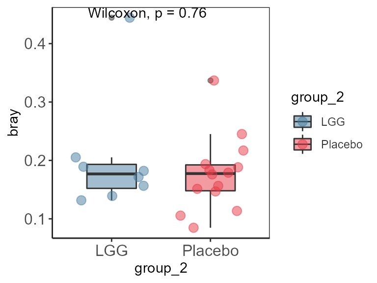
Area plot
Area plots can be used to visualize changes in abundances in
individual participants, or bioreactors sampled over time.
Here, we use a randomly chosen small subset of data from HMP2data.
library(microbiomeutilities)
library(RColorBrewer)
data("hmp2")
ps <- hmp2
ps.rel <- microbiome::transform(ps, "compositional")
# chose specific participants to plot data.
pts <- c("Participant_1","Participant_2",
         "Participant_8","Participant_5")
#pts <- "Participant_1"
ps.rel <- subset_samples(ps.rel, subject_id %in% pts)
p <- plot_area(ps.rel, xvar="visit_number",
               level = "Family",
               facet.by = "subject_id",
               abund.thres = 0.1,
               prev.thres=0.1,
               fill.colors=brewer.pal(12,"Paired"),
               ncol=2,
               nrow=2)
p + ylab("Relative abundance") +
  scale_y_continuous(labels = scales::percent)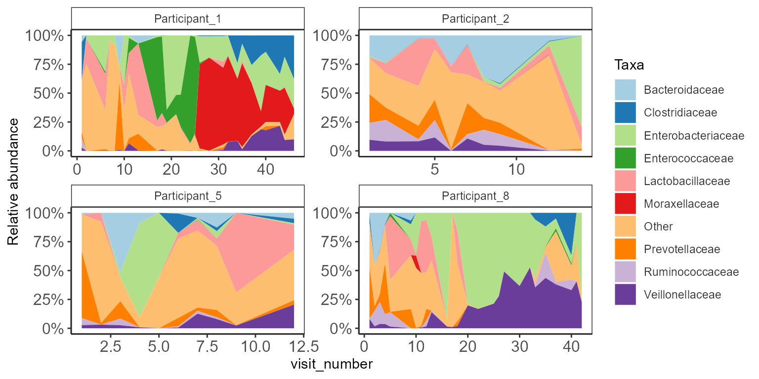
Paired abundances
We use a subset of HMP2 data
library(microbiome)
library(microbiomeutilities)
#library(gghalves)
library(tidyr)

data("hmp2")
ps <- hmp2
# pick visit 1 and 2
ps.sub <- subset_samples(ps, visit_number %in% c(1,2))
ps.sub <- prune_taxa(taxa_sums(ps.sub)>0, ps.sub)

ps.rel <- microbiome::transform(ps.sub, "compositional")
ps.rel.f <- format_to_besthit(ps.rel)

#top_taxa(ps.rel.f, 5)
# Check how many have both time points
table(meta(ps.rel.f)$visit_number)
#>
#>  1  2
#> 13 11
#table(meta(ps.rel.f)$visit_number, meta(ps.rel.f)$subject_id)
# there are two Participant_3 and Participant_11 with no time point2 sample

select.taxa <- c("4430843:g__Prevotella", "580629:g__Bacteroides")

group.colors = c("brown3", "steelblue", "grey70")


p <- plot_paired_abundances (ps.rel.f,
                             select.taxa=select.taxa,
                             group="visit_number",
                             group.colors=group.colors,
                             dot.opacity = 0.25,
                             dot.size= 2,
                             add.violin = TRUE,
                             line = "subject_id",
                             line.down = "#7209b7",
                             line.stable = "red",
                             line.up = "#14213d",
                             line.na.value = "red",
                             line.guide = "none",
                             line.opacity = 0.25,
                             line.size = 1)
print(p + xlab("Time point") + ylab("Relative abundance"))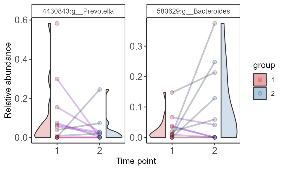
The lines are colored according to their change in abundance from time 1 to time 2.
Spaghetti plots
One participant many taxa
Reference for visualization and original code Data to
Viz.com
The ordering of panel on top of each other is better for comparisons. However, practical consideration can be made on number of columns and rows to distribute the panels.
library(microbiomeutilities)
data("hmp2")
pseq <- hmp2 # Ren
pseq.rel <- microbiome::transform(pseq, "compositional")
pseq.relF <- format_to_besthit(pseq.rel)

# Choose one participant
phdf.s <- subset_samples(pseq.relF, subject_id==
                           "Participant_1")
# Choose top 12 taxa to visualize
ntax <- top_taxa(phdf.s, 4)
phdf.s <- prune_taxa(ntax, phdf.s)

plot_spaghetti(phdf.s, plot.var= "by_taxa",
               select.taxa=ntax,
               xvar="visit_number",
               line.bg.color="#8d99ae",
               focus.color="brown3",
               focus.line.size = 1,
               ncol=1,
               nrow=4,
               line.size=0.2)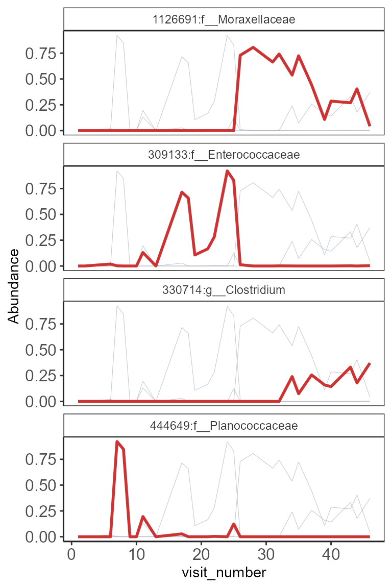
One taxa many participants
pseq.relF <- format_to_besthit(pseq.rel)
ntax2 <- core_members(pseq.relF, 0.001, 0.5)
# chose first for example
ntax2 # only
#> [1] "581782:f__Enterobacteriaceae"
# check how many participants are there in "subject_id"
length(unique(meta(pseq.relF)$subject_id))
#> [1] 13

# There are 13 participants. Choose ncol and nrow accordingly

plot_spaghetti(pseq.relF, plot.var= "by_sample",
               select.taxa=ntax2,
               group= "subject_id",
               xvar="visit_number",
               line.bg.color="#8d99ae",
               focus.color="brown3",
               focus.line.size = 1,
               ncol=4,
               nrow=6,
               line.size=0.2)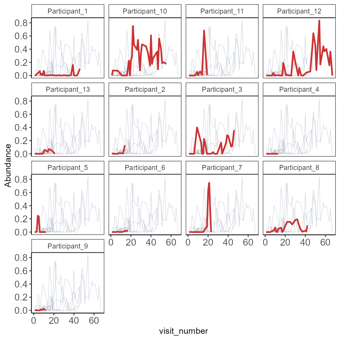
This package is part of the microbiomeverse tools.
See also microbiome
R/BioC package
Contributions are welcome:
Issue
Tracker
Pull
requests
Star us on the
Github page
sessionInfo()
#> R version 4.2.1 (2022-06-23 ucrt)
#> Platform: x86_64-w64-mingw32/x64 (64-bit)
#> Running under: Windows 10 x64 (build 19044)
#>
#> Matrix products: default
#>
#> locale:
#> [1] LC_COLLATE=English_United States.utf8
#> [2] LC_CTYPE=English_United States.utf8
#> [3] LC_MONETARY=English_United States.utf8
#> [4] LC_NUMERIC=C
#> [5] LC_TIME=English_United States.utf8
#>
#> attached base packages:
#> [1] stats     graphics  grDevices utils     datasets  methods   base
#>
#> other attached packages:
#> [1] tidyr_1.2.0                 RColorBrewer_1.1-3
#> [3] ggpubr_0.4.0                microbiomeutilities_1.00.16
#> [5] dplyr_1.0.9                 microbiome_1.18.0
#> [7] ggplot2_3.3.6               phyloseq_1.40.0
#>
#> loaded via a namespace (and not attached):
#>   [1] nlme_3.1-157           bitops_1.0-7           fs_1.5.2
#>   [4] gghalves_0.1.3         rprojroot_2.0.3        GenomeInfoDb_1.32.2
#>   [7] backports_1.4.1        tools_4.2.1            bslib_0.4.0
#>  [10] utf8_1.2.2             R6_2.5.1               vegan_2.6-2
#>  [13] DBI_1.1.3              BiocGenerics_0.42.0    mgcv_1.8-40
#>  [16] colorspace_2.0-3       permute_0.9-7          rhdf5filters_1.8.0
#>  [19] ade4_1.7-19            withr_2.5.0            tidyselect_1.1.2
#>  [22] compiler_4.2.1         textshaping_0.3.6      cli_3.3.0
#>  [25] Biobase_2.56.0         desc_1.4.2             labeling_0.4.2
#>  [28] sass_0.4.2             scales_1.2.1           pkgdown_2.0.6
#>  [31] systemfonts_1.0.4      stringr_1.4.1          digest_0.6.29
#>  [34] rmarkdown_2.16         XVector_0.36.0         pkgconfig_2.0.3
#>  [37] htmltools_0.5.3        highr_0.9              fastmap_1.1.0
#>  [40] rlang_1.0.5            rstudioapi_0.14        farver_2.1.1
#>  [43] jquerylib_0.1.4        generics_0.1.3         jsonlite_1.8.0
#>  [46] car_3.1-0              RCurl_1.98-1.6         magrittr_2.0.3
#>  [49] GenomeInfoDbData_1.2.8 biomformat_1.24.0      Matrix_1.5-1
#>  [52] Rcpp_1.0.8.3           munsell_0.5.0          S4Vectors_0.34.0
#>  [55] Rhdf5lib_1.18.2        fansi_1.0.3            abind_1.4-5
#>  [58] ape_5.6-2              lifecycle_1.0.2        stringi_1.7.6
#>  [61] yaml_2.3.5             carData_3.0-5          MASS_7.3-57
#>  [64] zlibbioc_1.42.0        rhdf5_2.40.0           Rtsne_0.16
#>  [67] plyr_1.8.7             grid_4.2.1             ggrepel_0.9.1
#>  [70] parallel_4.2.1         crayon_1.5.1           lattice_0.20-45
#>  [73] Biostrings_2.64.0      splines_4.2.1          multtest_2.52.0
#>  [76] knitr_1.40             pillar_1.8.1           igraph_1.3.1
#>  [79] ggsignif_0.6.3         reshape2_1.4.4         codetools_0.2-18
#>  [82] stats4_4.2.1           glue_1.6.2             evaluate_0.16
#>  [85] data.table_1.14.2      vctrs_0.4.1            foreach_1.5.2
#>  [88] gtable_0.3.1           purrr_0.3.4            assertthat_0.2.1
#>  [91] cachem_1.0.6           xfun_0.31              broom_1.0.1
#>  [94] rstatix_0.7.0          ragg_1.2.2             survival_3.3-1
#>  [97] pheatmap_1.0.12        tibble_3.1.7           iterators_1.0.14
#> [100] memoise_2.0.1          IRanges_2.30.0         cluster_2.1.3
#> [103] ellipsis_0.3.2